Continuous flow reactors are almost always operated at steady state. We will consider three types: the continuous-stirred tank reactor (CSTR), the plug flow reactor (PFR), and the packed-bed reactor (PBR). Detailed physical descriptions of these reactors can be found in both the Professional Reference Shelf (PRS) for Chapter 1 and in the Visual Encyclopedia of Equipment on the DVD-ROM.

Continuous-Stirred Tank Reactor (CSTR)
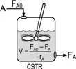
A type of reactor used commonly in industrial processing is the stirred tank operated continuously (Figure 1-7). It is referred to as the continuous-stirred tank reactor (CSTR) or vat, or backmix reactor, and is used primarily for liquid phase reactions. It is normally operated at steady state and is assumed to be perfectly mixed; consequently, there is no time dependence or position dependence of the temperature, concentration, or reaction rate inside the CSTR. That is, every variable is the same at every point inside the reactor. Because the temperature and concentration are identical everywhere within the reaction vessel, they are the same at the exit point as they are elsewhere in the tank. Thus, the temperature and concentration in the exit stream are modeled as being the same as those inside the reactor. In systems where mixing is highly nonideal, the well-mixed model is inadequate, and we must resort to other modeling techniques, such as residence-time distributions, to obtain meaningful results. This topic of nonideal mixing is discussed in DVD-ROM Chapters DVD13 and DVD14, on the DVD-ROM included with this text, and in Chapters 13 and 14 in the fourth edition of The Elements of Chemical Reaction Engineering (ECRE).
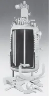
Figure 1-7(a) CSTR/batch reactor.
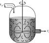
Figure 1-7(b) CSTR mixing patterns. Also see the Visual Encyclopedia of Equipment on the DVD-ROM.
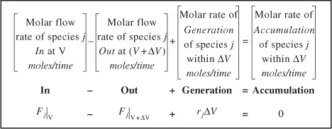
When the general mole balance equation
Equation 1-4

is applied to a CSTR operated at steady state (i.e., conditions do not change with time),

in which there are no spatial variations in the rate of reaction (i.e., perfect mixing),

The ideal CSTR is assumed to be perfectly mixed.
it takes the familiar form known as the design equation for a CSTR:
Equation 1-7
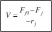
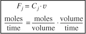
The CSTR design equation gives the reactor volume V necessary to reduce the entering flow rate of species j from Fj 0 to the exit flow rate Fj , when species j is disappearing at a rate of –rj . We note that the CSTR is modeled such that the conditions in the exit stream (e.g., concentration, and temperature) are identical to those in the tank. The molar flow rate Fj is just the product of the concentration of species j and the volumetric flow rate u:
Equation 1-8
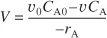
Similarly, for the entrance molar flow rate we have Fj0 = Cj0 · v0. Consequently, we can substitute for Fj 0 and Fj into Equation (1-7) to write a balance on species A as
Equation 1-9
The ideal CSTR mole balance equation is an algebraic equation, not a differential equation.
Tubular Reactor
In addition to the CSTR and batch reactors, another type of reactor commonly used in industry is the tubular reactor. It consists of a cylindrical pipe and is normally operated at steady state, as is the CSTR. Tubular reactors are used most often for gas-phase reactions. A schematic and a photograph of industrial tubular reactors are shown in Figure 1-8.
When is a tubular reactor most often used?
In the tubular reactor, the reactants are continually consumed as they flow down the length of the reactor. In modeling the tubular reactor, we assume that the concentration varies continuously in the axial direction through the reactor. Consequently, the reaction rate, which is a function of concentration for all but zero-order reactions, will also vary axially. For the purposes of the material presented here, we consider systems in which the flow field may be modeled by that of a plug flow profile (e.g., uniform velocity as in turbulent flow), as shown in Figure 1-9. That is, there is no radial variation in reaction rate, and the reactor is referred to as a plug-flow reactor (PFR). (The laminar flow reactor is discussed on the DVD-ROM in Chapter DVD13 and in Chapter 13 of the fourth edition of ECRE.)
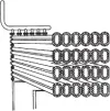
Figure 1-8(a) Tubular reactor schematic. Longitudinal tubular reactor. [Excerpted by special permission from Chem. Eng., 63 (10), 211 (Oct. 1956). Copyright 1956 by McGraw-Hill, Inc., New York, NY 10020.]
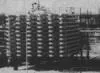
Figure 1-8(b) Tubular reactor photo. Tubular reactor for production of Dimersol
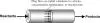
Figure 1-9 Plug-flow tubular reactor.
Also see PRS and Visual Encyclopedia of Equipment.
The general mole balance equation is given by Equation (1-4):
Equation 1-4
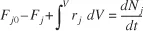
The equation we will use to design PFRs at steady state can be developed in two ways: (1) directly from Equation (1-4) by differentiating with respect to volume V, and then rearranging the result or (2) from a mole balance on species j in a differential segment of the reactor volume ΔV. Let’s choose the second way to arrive at the differential form of the PFR mole balance. The differential volume, ΔV shown in Figure 1-10, will be chosen sufficiently small such that there are no spatial variations in reaction rate within this volume. Thus the generation term, ΔGj, is
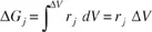
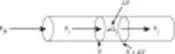
Figure 1-10 Mole balance on species j in volume Δ V.
Equation 1-10
Dividing by ΔV and rearranging
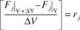
the term in brackets resembles the definition of a derivative
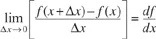
Taking the limit as ΔV approaches zero, we obtain the differential form of steady state mole balance on a PFR.
Equation 1-11

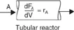
We could have made the cylindrical reactor on which we carried out our mole balance an irregular shape reactor, such as the one shown in Figure 1-11 for reactant species A.
Picasso’s reactor
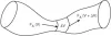
Figure 1-11 Pablo Picasso’s reactor.
However, we see that by applying Equation (1-10), the result would yield the same equation (i.e., Equation [1-11]). For species A, the mole balance is
Equation 1-12

Consequently, we see that Equation (1-11) applies equally well to our model of tubular reactors of variable and constant cross-sectional area, although it is doubtful that one would find a reactor of the shape shown in Figure 1-11 unless it were designed by Pablo Picasso.
The conclusion drawn from the application of the design equation to Picasso’s reactor is an important one: the degree of completion of a reaction achieved in an ideal plug-flow reactor (PFR) does not depend on its shape, only on its total volume.
Again consider the isomerization A ![]() B, this time in a PFR. As the reactants proceed down the reactor, A is consumed by chemical reaction and B is produced. Consequently, the molar flow rate F A decreases, while F B increases as the reactor volume V increases, as shown in Figure 1-12.
B, this time in a PFR. As the reactants proceed down the reactor, A is consumed by chemical reaction and B is produced. Consequently, the molar flow rate F A decreases, while F B increases as the reactor volume V increases, as shown in Figure 1-12.
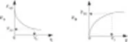
Figure 1-12 Profiles of molar flow rates in a PFR.

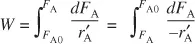
We now ask what is the reactor volume V 1 necessary to reduce the entering molar flow rate of A from F A0 to F A1. Rearranging Equation (1-12) in the form

and integrating with limits at V = 0, then F A = F A0, and at V = V 1, then F A = F A1.
Equation 1-13
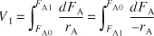
V1 is the volume necessary to reduce the entering molar flow rate FA0 to some specified value FA1 and also the volume necessary to produce a molar flow rate of B of FB1.
Packed-Bed Reactor (PBR)
The principal difference between reactor design calculations involving homogeneous reactions and those involving fluid-solid heterogeneous reactions is that for the latter, the reaction takes place on the surface of the catalyst (see Chapter 10). Consequently, the reaction rate is based on mass of solid catalyst, W, rather than on reactor volume, V. For a fluid–solid heterogeneous system, the rate of reaction of a species A is defined as
![]() = mol A reacted/(time x mass of catalyst)
= mol A reacted/(time x mass of catalyst)
The mass of solid catalyst is used because the amount of catalyst is what is important to the rate of product formation. The reactor volume that contains the catalyst is of secondary significance. Figure 1-13 shows a schematic of an industrial catalytic reactor with vertical tubes packed with solid catalyst.
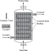
Figure 1-13 Longitudinal catalytic packed-bed reactor. [From Cropley, American Institute of Chemical Engineers, 86(2), 34 (1990). Reproduced with permission of the American Institute of Chemical Engineers,
PBR Mole Balance
In the three idealized types of reactors just discussed (the perfectly mixed batch reactor, the plug-flow tubular reactor [PFR]), and the perfectly mixed continuous-stirred tank reactor [CSTR]), the design equations (i.e., mole balances) were developed based on reactor volume. The derivation of the design equation for a packed-bed catalytic reactor (PBR) will be carried out in a manner analogous to the development of the tubular design equation. To accomplish this derivation, we simply replace the volume coordinate in Equation (1-10) with the catalyst mass (i.e., weight) coordinate W (Figure 1-14).
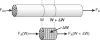
Figure 1-14 Packed-bed reactor schematic.
As with the PFR, the PBR is assumed to have no radial gradients in concentration, temperature, or reaction rate. The generalized mole balance on species A over catalyst weight ΔW results in the equation
Equation 1-14
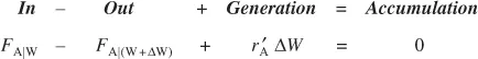
The dimensions of the generation term in Equation (1-14) are

which are, as expected, the same dimensions of the molar flow rate F A. After dividing by ΔW and taking the limit as ΔW ![]() 0, we arrive at the differential form of the mole balance for a packed-bed reactor:
0, we arrive at the differential form of the mole balance for a packed-bed reactor:
Equation 1-15

Use the differential form of design equation for catalyst decay and pressure drop.
When pressure drop through the reactor (see Section 5.5) and catalyst decay (see Section 10.7 in DVD-ROM Chapter 10) are neglected, the integral form of the packed-catalyst-bed design equation can be used to calculate the catalyst weight.

Equation 1-16
You can use the integral form only when there is no ΔP and no catalyst decay.
W is the catalyst weight necessary to reduce the entering molar flow rate of species A, F A0, down to a flow rate F A.
For some insight into things to come, consider the following example of how one can use the tubular reactor design in Equation (1-11).
Example 1–2. How Large Is It?
· Consider the liquid phase cis – trans isomerization of 2–butene
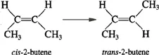
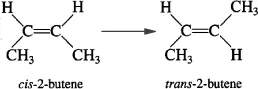
which we will write symbolically as

The reaction is first order in A (–r A = kC A) and is carried out in a tubular reactor in which the volumetric flow rate, v, is constant, i.e., v= v0.
· Sketch the concentration profile.
· Derive an equation relating the reactor volume to the entering and exiting concentrations of A, the rate constant k, and the volumetric flow rate v 0.
· Determine the reactor volume necessary to reduce the exiting concentration to 10% of the entering concentration when the volumetric flow rate is 10 dm3/min (i.e., liters/min) and the specific reaction rate, k, is 0.23 min–1.
Solution
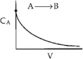
· Sketch C A as a function of V.
Species A is consumed as we move down the reactor, and as a result, both the molar flow rate of A and the concentration of A will decrease as we move. Because the volumetric flow rate is constant, v = v0, one can use Equation (1-8) to obtain the concentration of A, C A = F A/v0, and then by comparison with Figure 1-12 plot, the concentration of A as a function of reactor volume, as shown in Figure E1-2.1.
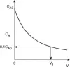
Figure E1-2.1 Concentration profile.
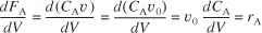
· Derive an equation relating V, v0, k, C A0, and C A.
For a tubular reactor, the mole balance on species A (j = A) was shown to be given by Equation (1-11). Then for species A (j = A)
Equation 1-12

For a first-order reaction, the rate law (discussed in Chapter 3) is
Equation E1-2.1

Reactor sizing
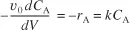
Because the volumetric flow rate, v, is constant (v = v0), as it is for most all liquid-phase reactions,
Equation E1-2.2
Multiplying both sides of Equation (E1-2.2) by minus one and then substituting Equation (E1-2.1) yields
Equation E1-2.3
Separating the variables and rearranging gives

Using the conditions at the entrance of the reactor that when V = 0, then C A = C A0,
Equation E1-2.4
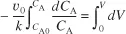
Carrying out the integration of Equation (E1-2.4) gives
Equation E1-2.5

We can also rearrange Equation (E1-2.5) to solve for the concentration of A as a function of reactor volume to obtain
C = C Aoexp(–kV/v0)
Concentration Profile
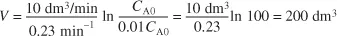
· Calculate V. We want to find the volume, V1, at which  for k = 0.23 min–1 and v0 = 10 dm3/min.
Substituting C A0, C A, v0, and k in Equation (E1-2.5), we have

Let’s calculate the volume to reduce the entering concentration to C A = 0.01 C A0. Again using equation (E1-2.5)

)
Comments are closed.